Calling Python Functions from kdb+/q with PyKX

PyKX allows you to call Python functions from kdb+/q (and vice versa), enabling powerful data analysis using the rich ecosystem of libraries available in Python. In this post, I will show how you can invoke a Lasso Regression function in Python by passing a table from a q script.

1. Install PyKX

pip install pykx

2. Create a Python (.p) file

Create a Python file called lasso.p containing a function that takes a Pandas DataFrame, performs Lasso regression (using the scikit-learn machine learning library), and returns a vector of coefficients.

# lasso.p

import numpy as np
import pandas as pd
from sklearn.linear_model import Lasso

def lasso_regression(df):
    X = df.iloc[:, :-1]
    y = df.iloc[:, -1]

    # Perform Lasso regression
    lasso = Lasso(alpha=0.1)
    lasso.fit(X, y)

    coefficients = np.append(lasso.coef_, lasso.intercept_) 
    return coefficients

3. Invoke the Python function from a q script

Next, write a q script that generates a table of random data and invokes the Python function with it.

// Load pykx and the python file
\l /path/to/python/site-packages/pykx/pykx.q
\l lasso.p

// Create a sample table with random x and y values
n:100;
x:n?10f;
y:2*x+n?2f;
data:([]x;y);

// Call the python function
qfunc:.pykx.get[`lasso_regression;<];
coefficients:qfunc data;

Conversion of data types between kdb+/q and Python

When transferring data between q and Python, PyKX applies "default" type conversions. For instance, tables in q are automatically converted to Pandas DataFrames, and lists are converted to NumPy arrays. You can call .pykx.setdefault to change the default conversion type to Pandas, Numpy, Python, or PyArrow. PyKX also provides functions to convert q data types to specific Python types, such as .pykx.tonp which tags a q object to be converted to a NumPy object. The following code illustrates type conversion:

q) .pykx.util.defaultConv
"default"

// lists are converted to NumPy arrays by default
q) .pykx.print .pykx.eval["lambda x: type(x)"] til 10
<class 'numpy.ndarray'>

// tables are converted to Pandas DataFrames by default
q) .pykx.print .pykx.eval["lambda x: type(x)"] ([] foo:1 2)
<class 'pandas.core.frame.DataFrame'>

// change default conversion to NumPy
q) .pykx.setdefault["Numpy"]

// tables are NumPy arrays now
q) .pykx.print .pykx.eval["lambda x: type(x)"] ([] foo:1 2)
<class 'numpy.recarray'>

// change default conversion to Python
q) .pykx.setdefault["Python"]

// tables are converted to dict when using Python conversion
q) .pykx.print .pykx.eval["lambda x: type(x)"] ([] foo:1 2)
<class 'dict'>

// tag a q object as a Pandas DataFrame
q) .pykx.print .pykx.eval["lambda x: type(x)"] .pykx.topd ([] foo:1 2)
<class 'pandas.core.frame.DataFrame'>

Linear and Polynomial Regression in kdb+/q

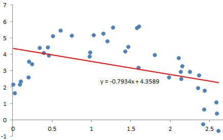
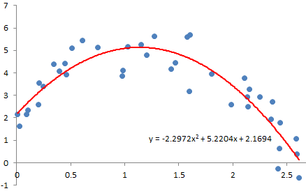
In this post, I'll describe how you can implement linear and polynomial regression in kdb+/q to determine the equation of a line of best fit (also known as a trendline) through the data on a scatter plot.

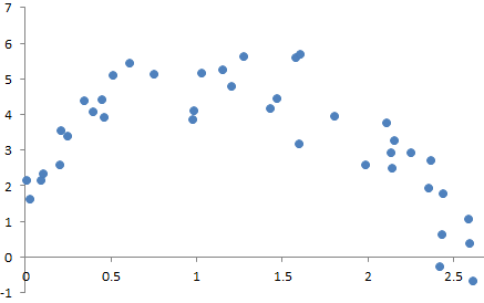
Consider the following scatter plot:

Our aim is to estimate a function of a line that most closely fits the data.

The vector of estimated polynomial regression coefficients (using ordinary least squares estimation) can be obtained using the following formula (for information about how this formula is derived, see Regression analysis [Wikipedia]):

b = (XTX)−1XTy

This can be translated into q as follows:

computeRegressionCoefficients:{
    xt:flip x;
    xt_x:xt mmu x;
    xt_x_inv:inv xt_x;
    xt_y:xt mmu y;
    xt_x_inv mmu xt_y}

Linear:
In order to perform linear regression, we have to first create a matrix X with a column of 1s and a column containing the x-values. The output of linear regression will be a vector of 2 coefficients and the equation of the trendline will be of the form: y = b1x + b0

computeLinearRegressionCoefficients:{
    computeRegressionCoefficients[flip (1f;x);y]}

Polynomial:
In order to fit a polynomial line, all we have to do is take the matrix X from the linear regression model and add more columns corresponding to the order of the polynomial desired. For example, for quadratic regression, we will add a column for x² on the right side of the matrix X. The output of quadratic regression will be a vector of 3 coefficients and the equation of the curve will be of the form: y = b2x2 + b1x + b0

// quadratic
computeQuadraticRegressionCoefficients:{
    computeRegressionCoefficients[flip (1f;x;x*x);y]}

// cubic
computeCubicRegressionCoefficients:{
    computeRegressionCoefficients[flip (1f;x;x*x;x*x*x);y]}

// generalisation of polynomial regression for any order
computePolynomialRegressionCoefficients:{[x;y;order]
    computeRegressionCoefficients[flip x xexp/: til order+1;y]}

Related post:
Matrix Operations in kdb+/q

Matrix Operations in kdb+/q

In q, a matrix (an array of m x n numbers) is represented as a list of lists. For example, here is a matrix with 2 rows and 3 columns:

q)A:(1 2 3;4 5 6)
q)A
1 2 3
4 5 6

Matrix Addition and Subtraction
If A and B are matrices of the same size, then they can be added and subtracted. To find the entries of A + B, you simply add the corresponding entries of A and B. To find A - B, subtract corresponding entries. If A and B have different sizes, you will get a 'length error.

q)A:(1 2;3 4)
q)B:(5 6;7 8)
q)A+B
6  8
10 12
q)B-A
4 4
4 4
q)C:(1 1 1;2 2 2)
q)A+C
'length
  [0]  A+C
        ^

Scalar Multiplication
If A is a matrix and k is a scalar, then the matrix kA is obtained by multiplying each entry of A by k.

q)A:(1 2;3 4)
q)k:2
q)k*A
2 4
6 8

Matrix Multiplication
First, in order to multiply two matrices A and B, the number of columns of A must match the number of rows of B. If A is m x n and B is n x p, then the size of the product matrix AB will be m x p. In order to calculate AB, you have to take the dot product (multiply corresponding numbers and then add them up) of each row vector in A and the corresponding column vector in B. This can be done in q using the mmu (or $) operator.

q)A:(1 2f;3 4f)
q)B:(5 6f;7 8f)
q)A
1 2
3 4
q)B
5 6
7 8
q)A mmu B
19 22
43 50

Identity Matrix
This is a square matrix with 1s on the diagonal and 0s everywhere else.

q)I:{`float${x=/:x}til x}
q)I 3
1 0 0
0 1 0
0 0 1

Matrix Inverse
The inverse of A is A^-1 if AA^-1=A^-1A=I, where I is the identity matrix. Use the inv function to find the inverse of a matrix.

q)A:(1 2f;3 4f)
q)inv A
-2  1
1.5 -0.5
q)A mmu inv A
1 1.110223e-016
0 1

Matrix Tranpose
The tranpose A^T of a matrix A is a flipped version of the original matrix which is obtained by changing its rows into columns (or equivalently, its columns into rows). This can be done by using the flip operation in q.

q)A:(1 2 3;4 5 6)
q)flip A
1 4
2 5
3 6

Upper Triangular Matrix
This is a square matrix in which all the entries below the main diagonal are zero.

q)upperTriangle:{`float${x<=\:x}til x}
q)upperTriangle 3
1 1 1
0 1 1
0 0 1

Lower Triangular Matrix
This is a square matrix in which all the entries above the main diagonal are zero.

q)lowerTriangle:{`float${x>=\:x}til x}
q)lowerTriangle 3
1 0 0
1 1 0
1 1 1

kdb+/q - Converting a CSV String into a Table

I often find myself wanting to create quick in-memory tables in q for testing purposes. The usual way to create a table is by specifying lists of column names and values, or flipping a dictionary, as shown below:

([] name:`Alice`Bob`Charles;age:20 30 40;city:`London`Paris`Athens)

// or, using a dictionary:

flip `name`age`city!(`Alice`Bob`Charles;20 30 40;`London`Paris`Athens)

As you can see, it's quite difficult to visualise the table being created using this approach. That's why I sometimes prefer to create a table from a multi-line CSV string instead, using the 0: operator, as shown below:

("SIS";enlist",") 0:
"name,age,city
Alice,20,London
Bob,30,Paris
Charles,40,Athens
"

name    age city
------------------
Alice   20  London
Bob     30  Paris
Charles 40  Athens

Note that you can also load from a CSV file:

("SIS";enlist",") 0: `$"/path/to/file.csv"

Related post:
kdb+/q - Reading and Writing a CSV File

kdb+/q - Display a Table as a Tree

This post shows how you can convert a keyed table to a hierarchical tree format in kdb+/q. This could be useful if you want to display data as a tree widget in a front-end.

Consider the following keyed table of world populations:

continent     country        city            | population
---------------------------------------------| ----------
North America United States  New York City   | 8550405
North America United States  Los Angeles     | 3971883
North America Mexico         Mexico City     | 8918653
Europe        United Kingdom London          | 9126366
Europe        Russia         Moscow          | 12195221
Europe        Russia         Saint Petersburg| 5383890
Africa        Nigeria        Lagos           | 14862000
Africa        Egypt          Cairo           | 9908788
Africa        Egypt          Giza            | 8800000
Asia          China          Shanghai        | 22315474
Asia          India          Mumbai          | 12691836
Asia          China          Beijing         | 11716620

We would like to display it as a tree of continent > country > city, as shown below (similar to a pivot table in Excel):

node                        | population
----------------------------| ----------
Total                       | 128441136
    Asia                    | 46723930
        China               | 34032094
            Shanghai        | 22315474
            Beijing         | 11716620
        India               | 12691836
            Mumbai          | 12691836
    Africa                  | 33570788
        Egypt               | 18708788
            Cairo           | 9908788
            Giza            | 8800000
        Nigeria             | 14862000
            Lagos           | 14862000
    Europe                  | 26705477
        Russia              | 17579111
            Moscow          | 12195221
            Saint Petersburg| 5383890
        United Kingdom      | 9126366
            London          | 9126366
    North America           | 21440941
        United States       | 12522288
            New York City   | 8550405
            Los Angeles     | 3971883
        Mexico              | 8918653
            Mexico City     | 8918653

In order to achieve this, we need to aggregate the data with different groupings, then combine the resultant tables and format it into a tree.

1. Grouping the data

First, we will add a dummy Total column to the table and then aggregate the table with the following groupings:

• Total
• Total, continent
• Total, continent, country
• Total, continent, country, city

The code for this is shown below:

// add Total column to the table. (td is a keyed table)
td:(`Total,keys[td]) xkey update Total:`Total from td;
keyCols:keys td;

// create a list of groupings
groupings:(1+til count keyCols) sublist\: keyCols;

// aggregate the table with each grouping
// this gives us a list of keyed tables (one per grouping)
tds:?[td;();;c!(sum;)each c:cols value td] each {x!x} each groupings;

// this step is optional but it's nice to sort each table on population
tds:`population xdesc'tds;

2. Joining the data

Next, we need to join the tables that were obtained as a result of the groupings. We do this by unkeying the tables and then using uj:

td:keyCols xkey (uj/) 0!'tds;

3. Formatting the data

Now let's add a Path column by concatenating the key columns:

td:![td;();0b;enlist[`Path]!enlist(`$sv';">";(string;(each;{x except `};(flip;enlist,keyCols))))];
td:(`Path,keyCols) xkey td;

This is what our tree looks like so far:

Path                                            Total continent     country        city            | population
---------------------------------------------------------------------------------------------------| ----------
Total                                           Total                                              | 128441136
Total>Asia                                      Total Asia                                         | 46723930
Total>Africa                                    Total Africa                                       | 33570788
Total>Europe                                    Total Europe                                       | 26705477
Total>North America                             Total North America                                | 21440941
Total>Asia>China                                Total Asia          China                          | 34032094
Total>Africa>Egypt                              Total Africa        Egypt                          | 18708788
Total>Europe>Russia                             Total Europe        Russia                         | 17579111
Total>Africa>Nigeria                            Total Africa        Nigeria                        | 14862000
Total>Asia>India                                Total Asia          India                          | 12691836
Total>North America>United States               Total North America United States                  | 12522288
Total>Europe>United Kingdom                     Total Europe        United Kingdom                 | 9126366
Total>North America>Mexico                      Total North America Mexico                         | 8918653
Total>Asia>China>Shanghai                       Total Asia          China          Shanghai        | 22315474
Total>Africa>Nigeria>Lagos                      Total Africa        Nigeria        Lagos           | 14862000
Total>Asia>India>Mumbai                         Total Asia          India          Mumbai          | 12691836
Total>Europe>Russia>Moscow                      Total Europe        Russia         Moscow          | 12195221
Total>Asia>China>Beijing                        Total Asia          China          Beijing         | 11716620
Total>Africa>Egypt>Cairo                        Total Africa        Egypt          Cairo           | 9908788
Total>Europe>United Kingdom>London              Total Europe        United Kingdom London          | 9126366
Total>North America>Mexico>Mexico City          Total North America Mexico         Mexico City     | 8918653
Total>Africa>Egypt>Giza                         Total Africa        Egypt          Giza            | 8800000
Total>North America>United States>New York City Total North America United States  New York City   | 8550405
Total>Europe>Russia>Saint Petersburg            Total Europe        Russia         Saint Petersburg| 5383890
Total>North America>United States>Los Angeles   Total North America United States  Los Angeles     | 3971883

4. Reordering the rows

The tree looks okay so far and you can stop there if you want but it would look better if child nodes were directly under their parents e.g. Shanghai should appear under China. In order to do this, we cannot simply use uj to combine our tables but we need to use the Over (/) accumulator to build the tree instead.

In order to get the row ordering correct, we add an id to each row, which will be a combination of the parent id and the row id. These id's look like this: 0, 0.0, 0.1, 0.1.1 etc. and will be used to sort the tree so that children appear under their parents.

Here is the final version of the code:

// Converts a table into a tree.
// @param td - a keyed table
// @param sortCol - the column to sort on
// @returns a table with a tree column
table2tree:{[td;sortCol]
    // add Total column to the table
    td:(`Total,keys[td]) xkey update Total:`Total from td;
    keyCols:keys td;

    // create a list of groupings
    groupings:(1+til count keyCols) sublist\: keyCols;

    // aggregate the table with each grouping
    // this gives us a list of keyed tables (one per grouping)
    tds:?[td;();;c!(sum;)each c:cols value td] each {x!x} each groupings;

    // sort the tables
    if[not null sortCol;tds:sortCol xdesc'tds];

    // initial tree only has the Total row
    tree:update id:"0",node:enlist "Total" from 0!first tds;

    // build the tree using the over accumulator
    tree:{[tree;td]
        keyCols:keys td;

        // join the parent id to the current table
        td:td lj k xkey ?[tree;();0b;{x!x}(k:-1_keyCols),`id];

        // update the id by concatenating the parent id to the row id
        // we need to left-pad the row id so that sorting works correctly
        // e.g. 1.3 should come before 1.10
        td:update id:`$"."sv'flip(string id;(-1*count string count td)$string i) from td;

        // add a node column which corresponds to the value of the last key column
        td:![td;();0b;enlist[`node]!enlist last keyCols];

        // add indentation to the node based on the depth (i.e. number of key columns)
        indentation:(4*-1+count keyCols)#" ";
        td:update node:(indentation,/:string node) from td;

        // now add the table to tree
        tree uj 0!td
	}/[tree;1_tds];

    // sort the tree on id
    (`node,keyCols) xkey `id xasc tree}

This is what our final tree looks like:

q) data:3!("SSSI";enlist",") 0: `$"population.csv";
q) select node,population from table2tree[data;`population]

node                         population
-----------------------------------------
Total                        128441136
    Asia                     46723930
        China                34032094
            Shanghai         22315474
            Beijing          11716620
        India                12691836
            Mumbai           12691836
    Africa                   33570788
        Egypt                18708788
            Cairo            9908788
            Giza             8800000
        Nigeria              14862000
            Lagos            14862000
    Europe                   26705477
        Russia               17579111
            Moscow           12195221
            Saint Petersburg 5383890
        United Kingdom       9126366
            London           9126366
    North America            21440941
        United States        12522288
            New York City    8550405
            Los Angeles      3971883
        Mexico               8918653
            Mexico City      8918653

I also played around with adding lines to connect nodes of the tree but it got complicated very fast!

Can you think of a better way to do this? Let me know in the comments below!

Kdb+/q - File Compression

Large tables can be compressed in Kdb+ by setting .z.zd. Compression of data can reduce disk cost and in some cases even improve performance for applications that have fast CPUs but slow disks.

.z.zd is a list of three integers consisting of logical block size, algorithm (0=none, 1=q, 2=gzip, 3=snappy, 4=lz4hc) and compression level.

Here is an example showing how to compress a table:

// Helper function that sets .z.zd and
// returns the previous value of .z.zd
.util.setZzd:{
  origZzd:$[count key `.z.zd;.z.zd;()];
  if[x~();
    system"x .z.zd";
    :origZzd;
  ];
  .z.zd:x;
  origZzd}

// create a table
td:([]a:1000000?10; b:1000000?10; c:1000000?10);

// save the table to disk without compression
`:uncompressed set td;

// save the table to disk using q IPC compression
origZzd:.util.setZzd[(17;1;0)];
`:compressed set td;
.util.setZzd[origZzd];

You can check compression stats by using the -21! function:

q)-21!`:compressed
compressedLength  | 5747890
uncompressedLength| 24000041
algorithm         | 1i
logicalBlockSize  | 17i
zipLevel          | 0i

The size of the file on disk is reduced from 22.8 MB to 5.5 MB after using q IPC compression.

kdb+/q - Try Catch

Programming languages typically have a try-catch mechanism for dealing with exceptions. The try block contains the code you want to execute and the catch block contains the code that will be executed if an error occurs in the try block.

Here is an example of a simple try-catch block in Java, which attempts to parse a string into an int and returns -1 if there is an error.

try {
    return Integer.parseInt(x);
} catch (NumberFormatException e) {
    e.printStackTrace();
    return -1;
}

In this post, I will describe the try-catch equivalent for exception handling in the q programming language.

.Q.trp[f;x;g] - for unary functions

For unary functions, you can use .Q.trp (Extend Trap), which takes three arguments:

1. f - a unary function to execute
2. x - the argument of f
3. g - a function to execute if f fails. This function is called with two arguments, the error string x and the backtrace object y

For example:

// Define a function which casts a string to int
parseInt:{[x] "I"$x}

// Define an error function which prints the stack trace and returns -1
// Note: .Q.sbt formats the backtrace object and 2@ prints to stderr
g:{[x;y] 2@"Error: ",x,"\nBacktrace:\n",.Q.sbt y;-1i}

// Try calling the function (wrapped by .Q.trp) with a valid argument
.Q.trp[parseInt;"123";g]
123i

// Try calling the function (wrapped by .Q.trp) with an invalid argument
// The error function is called and the stack trace is printed
.Q.trp[parseInt;`hello;g]
Error: type
Backtrace:
  [2]  parseInt:{[x] "I"$x}
                        ^
  [1]  (.Q.trp)

  [0]  .Q.trp[parseInt;`hello;g]
       ^
-1i

Note: An alternative is to use Trap At which has syntax @[f;x;e] but you won't get the backtrace, so it's better to use .Q.trp.

.[f;args;e] - for n-ary functions

.Q.trp only works for unary functions. For functions with more than one argument, you need to use Trap which has the syntax .[f;args;e]. The error function e does not take any arguments, which means no backtrace available. For example:

// Define a ternary function that sums its arguments
add:{[x;y;z] x+y+z}

.[add;1 2 3;{2@"Failed to perform add";-1}]
6

.[add;(1;2;`foo);{2@"Failed to perform add\n";-1}]
Failed to perform add
-1

kdb+/q - Running a function multiple times and concatenating results

Let's say that you have a q function that you want to run for multiple inputs (for example, a list of dates) and you want to concatenate the outputs of each function call into a single table. This is demonstrated below:

// A function that returns some data for a single date.
getData:{[dt]
    t:select from data where date=dt;
    // do some more stuff
    t}

// list of dates
dates:2016.01.01+til 10

// call the function for each date and join results
result:(uj/) getData each dates;

// or, if you want to do some processing after each function call:
result:(uj/) {[dt;param]
    t:getData[dt];
    // do some stuff with param
    t}[;`foo] each dates;

kdb+/q - Joins

You're probably familiar with SQL joins, which are used to combine data from more than one table. This post shows how you can do the same in kdb.

I'll use the following two tables to demonstrate joins in kdb:

q) show age:([] name:`alice`charlie`dave`frank; age:25 26 31 33)
name    age
-----------
alice   25
charlie 26
dave    31
frank   33

q) show work:([] name:`alice`bob`charlie`eve; dept:`ops`dev`hr`eng)
name    dept
------------
alice   ops
bob     dev
charlie hr
eve     dev

Now let's join these tables on the name field using the different kinds of kdb joins:

Left Join (lj):

In a left join, all the rows of the left table are preserved, and those from the right table are only combined if the values in the key columns match those in the left table. If there are values in the left table that don't exist in the right, the joined columns will contain nulls.

q) age lj `name xkey work
name    age dept
----------------
alice   25  ops
charlie 26  hr
dave    31
frank   33

Union Join (uj):

A union join (referred to as a full outer join in SQL) returns rows from both tables, regardless of whether there is a match. If there is a match, it returns combined rows, and if there isn't, the missing side will contain nulls.

q) (`name xkey age) uj `name xkey work
name   | age dept
-------| --------
alice  | 25  ops
charlie| 26  hr
dave   | 31
frank  | 33
bob    |     dev
eve    |     eng

Inner Join (ij):

An inner join returns only those rows where there is a match in both tables.

q) age ij `name xkey work
name    age dept
----------------
alice   25  ops
charlie 26  hr

Equi Join (ej):

This is an inner join in which you can specify the list of columns to join on.

q) ej[`name;age;work]
name    age dept
----------------
alice   25  ops
charlie 26  hr

Plus Join (pj):

This is a left join, which also sums the values of common columns (other than key columns). This type of join doesn't exist in SQL.

q) t1:([] name:`alice`charlie`dave`frank; x:1 2 3 4)
q) t2:([] name:`alice`bob`charlie`eve; x:10 10 10 10)
q) t1 pj `name xkey t2
name    x
----------
alice   11
charlie 12
dave    3
frank   4

Cross Join (cross):

This is a "cartesian product". It joins everything to everything and isn't normally the kind of join people are looking for. Each row is a combination of the rows of the first and second table, so can be a dangerous join to run against large tables.

q) `name xasc work cross age
name    dept age
----------------
alice   ops  25
alice   dev  25
alice   hr   25
alice   eng  25
charlie ops  26
charlie dev  26
charlie hr   26
charlie eng  26
dave    ops  31
dave    dev  31
dave    hr   31
dave    eng  31
frank   ops  33
frank   dev  33
frank   hr   33
frank   eng  33

kdb+/q - Concatenating columns

This post shows how you can concatenate values in two or more columns of a table in kdb, into a single value. Consider the following table:

q) person:([] firstName:`Alice`Bob`Charles;lastName:`Smith`Jones`Brown)
q) person
firstName lastName
------------------
Alice     Smith
Bob       Jones
Charles   Brown

In SQL, it's quite easy to concatenate columns, like this:

SQL> select firstName || ' ' || lastName as fullName from person;
fullName
--------
Alice Smith
Bob Jones
Charles Brown

In q, the same thing can be achieved by flipping the firstName and lastName columns and then calling sv to convert the resulting vector into a string, using a space separator. This is shown below:

q) select fullName:`$" "sv'string flip(firstName;lastName) from person

// in functional form:
q) colsToJoin:`firstName`lastName;
q) ?[person;();0b;enlist[`fullName]!enlist(`$sv';" ";(string;(flip;(enlist,colsToJoin))))]

// if there are many repeated names, you can use .Q.fu to improve performance:
q) select fullName:.Q.fu[{`$" "sv'string x};flip(firstName;lastName)] from person

// in functional form, with .Q.fu:
q) ?[person;();0b;enlist[`fullName]!enlist(.Q.fu;{`$" "sv'string x};(flip;(enlist,colsToJoin)))]

kdb+/q - Reading and Writing a CSV File

This post shows how you can load a CSV file into kdb and write a table out from kdb to a CSV file.

Reading a CSV file:

Let's say that you'd like to load a file containing comma-separated values into an in-memory table in kdb. For example, here's my CSV file, which contains country populations (source: Worldometers):

$ head -5 worldPopulation.csv
region,country,population
Africa,Algeria,40375954
Africa,Angola,25830958
Africa,Benin,11166658
Africa,Botswana,2303820

My file has got two string columns and one integer column.

I can load it into kdb using the Zero Colon function: (types; delimiter) 0: filehandle

q) data:("SSI";enlist",") 0: `$"/path/to/worldPopulation.csv"
// "SSI" creates 2 symbol columns and one integer column

// let's look at the column types
q) meta data
c         | t f a
----------| -----
region    | s
country   | s
population| i

// check the data
q) 5#data
region country                  population
------------------------------------------
Africa Algeria                  40375954
Africa Angola                   25830958
Africa Benin                    11166658
Africa Botswana                 2303820
Africa Burkina Faso             18633725

// you can use * if you want string columns, instead of symbol ones
q) data:("**I";enlist",") 0: `$"/path/to/worldPopulation.csv"

q) meta data
c         | t f a
----------| -----
region    | C
country   | C
population| i

q) 5#data
region   country        population
----------------------------------
"Africa" "Algeria"      40375954
"Africa" "Angola"       25830958
"Africa" "Benin"        11166658
"Africa" "Botswana"     2303820
"Africa" "Burkina Faso" 18633725

Writing a CSV file:

To save a table to a CSV file, you can use the command: filehandle 0: delimiter 0: table

// first, let's try printing out the csv data to console
q) "," 0: data
"region,country,population"
"Africa,Algeria,40375954"
"Africa,Angola,25830958"
"Africa,Benin,11166658"
"Africa,Botswana,2303820"

// save it
q)(`$"/tmp/out.csv") 0: "," 0: data
`/tmp/out.csv